An interactive visualisation of immersed surfaces on Desmos

Note: this article is currently a WIP.

Some examples of surface visualisations

Here are a couple of versions of the Desmos save file with different cool pre-loaded plots:

• The default: a hemisphere (select the second plot for a full sphere)
• A mobius band
• A heliocoid
• An immersed Klein bottle in ${\mathbb{R}}^3$ (thanks to cFOURbon for entering the formula)
• A heart-shaped surface
• A shell (thanks to Kevin D. for the help and idea)
• Give me my chemistry degree immediately?

Note: The below was submitted as my essay for the final assignment in the unit MTH3110 - differential geometry, at Monash University, in Semester 1, 2021. I’ve chosen to upload it here for those who may have seen my Desmos surface visualisation, and are interested in how I derived it! However, it assumes familiarity, especially near the end, with differential-geometric quantities such as maps of surfaces and their derivatives, and tangent spaces.

The explanation and geometry of the Desmos visualisation

Here is an interactive visualisation of surfaces on Desmos (a graphing website), made by me. It takes a (continuous) function $f:U\to \mathbb{R}$, for some $U\subseteq {\mathbb{R}}^2$, and plots a projection of the graph of $f$ onto ${\mathbb{R}}^2$ as a “wire-frame”; it can also take a parametrisation $\sigma :U\to {\mathbb{R}}^3$ and plot a projection of its image in the plane.¹ We discuss the algebra and geometry used in its construction, and some geometric properties of the projection map. Henceforth, let us assume that $U$ is open, $f$ is a smooth function, and that $\sigma$ is a regular surface patch.

Projecting down to a plane

There are many ways to project ${\mathbb{R}}^3$, onto ${\mathbb{R}}^2$. However, a way to choose a sensible, well-behaved projection is to choose a plane $\mathrm{\Pi }$ through the origin (a linear subspace of ${\mathbb{R}}^3$), and perform an orthogonal projection ${\pi }^{\prime }$. Such a plane can be uniquely determined by using spherical coordinates. Consider an “observer” at $N\in S^2$, the unit sphere, and a standard map $\tau :{\mathbb{R}}^2\to S^2$ given by

here, $(u,v)$ respectively measure latitude and longitude.² The unit vectors in $T_0{\mathbb{R}}^3$ (denoting possible directions from the origin) are precisely points on $S^2$. Thus, we may take $\mathrm{\Pi }$ as the orthogonal complement of the span of $\{N\}$.

A fact from differential geometry is that $T_N{S}^2=\{v\in {\mathbb{R}}^3:N\cdot v=0\}$. If $v\in \mathrm{\Pi }$, then for any $kN\in \mathrm{span}\{N\}$ (where $k\in \mathbb{R}$), $(kN)\cdot v=k(N\cdot v)=0$. In particular, $N\cdot v=0$, so $v\in T_N{S}^2$. Conversely, a vector $v\in T_N{S}^2$ satisfies $(kN)\cdot v=k(N\cdot v)=0$ for all $k\in \mathbb{R}$, so $v\in \mathrm{\Pi }$. This means that $\mathrm{\Pi }=T_N{S}^2$, and $N$ is normal to this tangent space.

Next, we consider the problem of projecting from ${\mathbb{R}}^3$ into $\mathrm{\Pi }$ (and then into ${\mathbb{R}}^2$). Given an orthonormal basis $b=\{b_1,b_2\}$ for $\mathrm{\Pi }$ that extends to a right-handed orthonormal basis $b^{\prime }=\{b_1,b_2,N\}$ of ${\mathbb{R}}^3$, where $N=b_1\times b_2$, consider the orthogonal projection ${\pi }^{\prime }:{\mathbb{R}}^3\to \mathrm{\Pi }$. Since $\ker {\pi }^{\prime }={\mathrm{\Pi }}^{\perp }$ and $\pi {|}_{\mathrm{\Pi }}$ is the identity, it follows that ${\pi }^{\prime }(b_1)=b_1$, ${\pi }^{\prime }(b_2)=b_2$, and ${\pi }^{\prime }(N)=0$. The map ${\pi }^{\prime }$ is linear, so its matrix with respect to the bases $b^{\prime },b$ is

The geometry of this map is as follows: take a point $p\in {\mathbb{R}}^3$. Then the coset $p+{\mathrm{\Pi }}^{\perp }=\{p+kN:k\in \mathbb{R}\}$, a line parallel to $N$ (thus orthogonal to $\mathrm{\Pi }$) passing through $p$, is collapsed onto a point ${\pi }^{\prime }(p)\in \mathrm{\Pi }$; distinct parallel lines are collapsed to distinct points. This is an orthographic projection, where the axes are not foreshortened, that is, no length distortion due to perspective (see Figure~\mathbb Ref{fig:cylinder_perspective}).\footnote{See explanation of perspective and foreshortening in art.} Under this projection, we consider ${\mathbb{R}}^3$ as the quotient ${\mathbb{R}}^3/{\mathrm{\Pi }}^{\perp }$, and cannot distinguish between points on the same line parallel to ${\mathrm{\Pi }}^{\perp }$; the map has rank $2$ and nullity $1$.

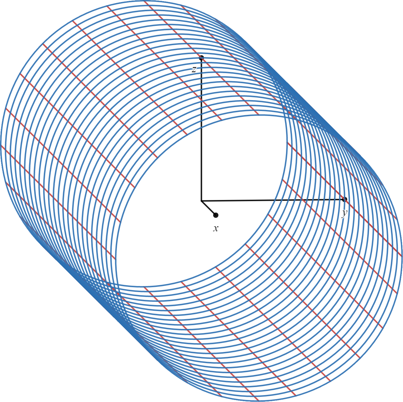
\begin{figure}[p!] \centering \includegraphics[width=0.75\textwidth]{cylinderperspective.png} \caption{Plot of cylinder $\sigma :(0,2\pi )\times (-4,4)\to S$, $\sigma (u,v)=(v,\cos u,\sin v)$ with perspective $(\theta ,\varphi )=(0.1,-0.1)$, using the Desmos visualisation. Observe that there is no distortion due to perspective (i.e. _foreshortening) in the negative $x$-direction.} \label{fig:cylinder_perspective} \end{figure}

Next, we consider the map that transforms points on $\mathrm{\Pi }$ into points in ${\mathbb{R}}^2$. Given our basis $b$ for $\mathrm{\Pi }$, there is a natural sense in which $b_1$ can be thought of as pointing “right”, and $b_2$ as pointing “up”. This is described by $T:\mathrm{\Pi }\to {\mathbb{R}}^2$, the linear isometry such that $T(b_1)=e_1$ and $T(b_2)=e_2$. Letting $e^{\prime }=\{e_1,e_2\}\subseteq {\mathbb{R}}^2$, $T$ is simply the identity in coordinates $b,e^{\prime }$: $T_{b,e^{\prime }}=I_2$, the $2\times 2$ identity matrix.

Thus, our overall projection $\pi :{\mathbb{R}}^3\to {\mathbb{R}}^2$ in the direction of $\mathrm{\Pi }$ would be given by $\pi =T\circ {\pi }^{\prime }$, with matrix $T_{b,e^{\prime }}{\pi }_{b^{\prime },b}^{\prime }$. However, we wish to express the matrix for $\pi$ with respect to the standard basis $e=\{e_1,e_2,e_3\}$ for ${\mathbb{R}}^3$. For this, we recall that the change-of-basis matrix from $b^{\prime }$ to $e$ is given by

Since $b^{\prime }$ is an orthonormal set, it follows that $M_{b^{\prime }\to e}\in O(3)$, so $M_{e\to b^{\prime }}=(M_{b^{\prime }\to e}{)}^{-1}=(M_{b^{\prime }\to e}{)}^{\mathrm{\top }}$. It follows that the matrix for $\pi$ w.r.t. the bases $e,e^{\prime }$ of ${\mathbb{R}}^3,{\mathbb{R}}^2$ respectively is

Now, recall that there is a pair $(\theta ,\varphi )$ corresponding to $N=\tau (\theta ,\varphi )$. For simplicity, we will assume that $\theta \in (-\pi /2,\pi /2)$, so that a suitable restriction of $\tau$ forms a regular chart for $S^2$. We aim to find an orthonormal basis for $\mathrm{\Pi }$ by finding an orthonormal basis for $T_N{S}^2$. Note that $\{{\tau }_u,{\tau }_v\}$ forms a basis for $T_N{S}^2$, where

and

It is easy to check that these are orthogonal, so an orthonormal basis $\{b_1,b_2\}$ for $\mathrm{\Pi }$ is found by normalising these vectors, yielding

and

(It turns out that this also works when $\theta \in \{\pm \pi /2\}$; these span the tangent planes $T_{(0,0,\pm 1)}{S}^2={\mathbb{R}}^2\times \{0\}$!) Note that we needed to take $b_1={\tau }_v/\Vert {\tau }_v\Vert$ and $b_2={\tau }_u/\Vert {\tau }_u\Vert$, so that indeed $b_1\times b_2=N=\tau (\theta ,\varphi )$.

In summary, for our perspective given by spherical coordinates $(\theta ,\varphi )$ (or equivalently $N=\tau (\theta ,\varphi )\in S^2$), the projection $\pi :{\mathbb{R}}^3\to {\mathbb{R}}^2$ is given by

Visualising the surface in Desmos

If we wish to plot $S$ as the graph of $f$, take $\sigma (u,v)=(u,v,f(u,v))$. Then it reduces to the problem of plotting the image of $\sigma$, or at least its projection under $\pi$. It would be useless (given limitations on Desmos) to present a filled-in outline—we would get a single splotch of colour (with jagged edges)! Instead, we use the idea that the domain $U$ is an open subset of ${\mathbb{R}}^2,$\footnote{Desmos does not like strict inequalities, so they are often closed subsets instead, but we can ignore the boundary of $U$.} and for fixed $(u,v)\in U$, we consider the curves $x_u,y_v:I_u,J_v\to U$ in $U$ (for suitable open intervals $I_u,J_v$), where $x_u(t)=(u,t)$ and $y_v(t)=(t,v)$, i.e. we fix the $u$ or $v$ coordinate, and let the other vary.

Consider a set of points $\{(u_i,v_i){\}}_i\subseteq U$, and the families of curves $\{x_{u_i}{\}}_i,\{y_{v_i}{\}}_i$ so-defined. Then for each of the curves (generically called $\alpha :I\to U$), we plot the image of $\gamma =\sigma \circ \alpha :I\to S$, a curve in $S$, under the projection $\pi$, yielding two families $\{\pi \circ \sigma \circ x_{u_i}{\}}_i$ (fixing $(x=)u=u_i$, plotted in red) and $\{\pi \circ \sigma \circ y_{v_i}{\}}_i$ (fixing $(y=)v=v_i$, plotted in blue) of curves in ${\mathbb{R}}^2$, representing moving along $S$ using $\sigma$, with one input fixed. In the visualisation, we assume that $U=(a_1,a_2)\times (b_1,b_2)$ is a box,\footnote{Technically $U=[a_1,a_2]\times [b_1,b_2]$, so we have a surface with boundary… but we can ignore this, as mentioned earlier.} and take $n_1,n_2$ curves of constant separation in $U$ in each direction. This creates the desired projection of the “wire-frame” on $S$, and varying $(\theta ,\varphi )$ allows us to visualise the plot of $S$ from all angles, giving it a 3-dimensional effect.

Differential geometry of the projection: changing perspective

For spherical coordinates $(\theta ,\varphi )$, let principal latitude denote ${\theta }_0\in [-\pi /2,\pi /2]$ such that there is ${\varphi }_0\in \mathbb{R}$ with $\tau (\theta ,\varphi )=\tau ({\theta }_0,{\varphi }_0)$. We see that $M(\theta ,\varphi )$ is a smooth function of $\theta ,\varphi$, so the matrix (and projection) smoothly varies with $\theta ,\varphi$:

and

Fixing a point $p=(x,y,z)\in {\mathbb{R}}^3$, we can think of $\pi$ as a function ${\mathbb{R}}^2\to {\mathbb{R}}^2$, where the inputs are spherical coordinates $(\theta ,\varphi )$; let us call this map ${\pi }^{\prime }:{\mathbb{R}}^2\to {\mathbb{R}}^2$, $(\theta ,\varphi )\mapsto \pi (p)=M(\theta ,\varphi )p$. Then the directional derivatives of ${\pi }^{\prime }$ are given by $D_{(\theta ,\varphi )}{\pi }^{\prime }:T_{(\theta ,\varphi )}{\mathbb{R}}^2\to T_{{\pi }^{\prime }(\theta ,\varphi )}{\mathbb{R}}^2$, which is such that

So, if we change perspective from $(\theta ,\varphi )$ with velocity $(\lambda ,\mu )\in T_{(\theta ,\varphi )}{\mathbb{R}}^2$ (i.e. increasing latitude by $\lambda$ and longitude by $\mu$), the image of $p$ in ${\mathbb{R}}^2$ moves with velocity $D_{(\theta ,\varphi )}{\pi }^{\prime }(\lambda ,\mu )$, given explicitly above. Note that

this relates the directional derivatives of ${\pi }^{\prime }$ to the partial derivatives of $M$.

Let us consider what happens to $\pi (p)$ when we fix longitude $\varphi$ and vary latitude $\theta$. Taking $\lambda =1$ and $\mu =0$ reveals a directional derivative of

in the $(1,0)$ direction. In particular, the $x$-coordinate of $\pi (p)$ does not change when only $\theta$ is changed, which makes sense since we view this as tilting the plane $\mathrm{\Pi }$ up or down. However, the $y$-coordinate changes at a rate precisely equal to $-\tau (\theta ,\varphi )\cdot p=-N\cdot p=\tau (-\theta ,\varphi +\pi )\cdot p$ (since $\tau$ gives points on $S^2$). For nonzero $p$, this is zero precisely when $p$, or equivalently $p/\Vert p\Vert \in S^2$, is orthogonal to $N\in S^2$, the unit normal vector to the plane of projection $\mathrm{\Pi }$. This holds when $N\in T_{p/\Vert p\Vert }{S}^2$; if $\tau (\mathbb{R}\times \{\varphi \})\subseteq T_{p/\Vert p\Vert }{S}^2$, then this occurs for every latitude $\theta$, but otherwise, $\tau (\mathbb{R}\times \{\varphi \})$ is a circle on $S^2$ and intersects $T_{p/\Vert p\Vert }{S}^2$ for precisely one latitude $\theta$ (modulo $\pi$). From this, we conclude that for principal latitudes $\theta$, if $p/\Vert p\Vert =\pm (N\times \tau (\theta +\pi /4,\varphi ))$, $\pi (p)$ is always fixed when varying latitude $\theta$ (the directional derivative is zero); otherwise, there is precisely one latitude $\theta$ (or two, whence $\theta =\pm \pi /2$) for which $\pi (p)$ has velocity zero.

The above observations agree with a direct calculation: the curve in ${\mathbb{R}}^2$ that $\pi (p)$ traces for fixed longitude $\varphi$ is

Now, let us consider what happens to $\pi (p)$ when we fix latitude $\theta$ and vary longitude $\varphi$. Taking $\lambda =0$ and $\mu =1$ gives a directional derivative of

in the $(0,1)$ direction. A direct calculation gives that the curve in ${\mathbb{R}}^2$ that $\pi (p)$ traces for fixed latitude $\theta$ is

the above directional derivative is simply ${\dot{\delta }}_p(\varphi )$. By trigonometry, we know that letting $T=t+{\cos }^{-1}(y/\sqrt{x^2+y^2})$,

this is clearly an ellipse (with period $2\pi$) with axis lengths $\sqrt{x^2+y^2}$ and $|\sin \theta |\sqrt{x^2+y^2}$, oriented negatively (clockwise) whenever principal latitude is positive (and positively if principal latitude is negative). Additionally, it has 4 vertices by Example 6.3 of chapter 4 (as long as $|\sin \theta |\ne 1$ and both axis lengths are nonzero); these vertices correspond to locations where the $x$ or $y$-coordinate of $\pi (p)$ is greatest or smallest. In summary, we see that for fixed latitude $\theta$, projected points move in an elliptic shape (in a clockwise direction when viewed from with positive principal latitude); this agrees with the intuition that as we increase longitude $\varphi$, in order for the normal $N$ to the plane of projection $\mathrm{\Pi }$ to point “into the screen”, points must rotate clockwise about the projected $z$-axis.

This concludes our analysis of the 2-dimensional visualisation of surfaces in ${\mathbb{R}}^3$ on Desmos. We saw some commentary on the derivation of the projection, using some linear algebra. Then we proceeded to analyse how curves are represented in the plot, as a “wire-frame”, and finally, we analysed the effect of changing latitude and longitude on the positions of points in the plot, rounding off a treatment of the algebraic, analytic, and geometric properties of the visualisation.

Acknowledgements

I would like to acknowledge Dan Mathews for giving useful feedback (especially with respect to interpreting the effect on changing perspective on the position of points) and verifying the procedure used to derive the projection matrix. Errors in my initial formula for the projection were also corrected through discussion and testing with various members of the Maths @ Monash Discord server.